Developing a Model in the Galactic Grams PLS/IQ Environment
In order to develop models in the Galactic Grams environment one must have a full Grams 32 software package with the PLS/IQ add-on. The first thing that one must do, however, is get all the lab data into an excel spreadsheet and associate that data with a galactic spectrum file (SPC file – *.spc). Initially, about 50-150 samples are analyzed in the laboratory and sub samples are sent to Process NMR Associates for NMR analysis. The chemometric models developed on these initial samples are used as the starting models when the system is installed. After installation the model is tuned and expanded to cover the full operational conditions of the process unit. This model-tuning can be done either by a concerted sample gathering effort or by simply “piggy-backing” onto the existing sampling schedule. What is of vital importance is that the actual time that the sample is grabbed is associated with that sample when it is placed in the plants LIMS system for lab analysis. Having the actual sampling time allows the correct spectrum to be used in the modeling when the data is provided for model update.
Once the data has been placed in an excel spreadsheet:
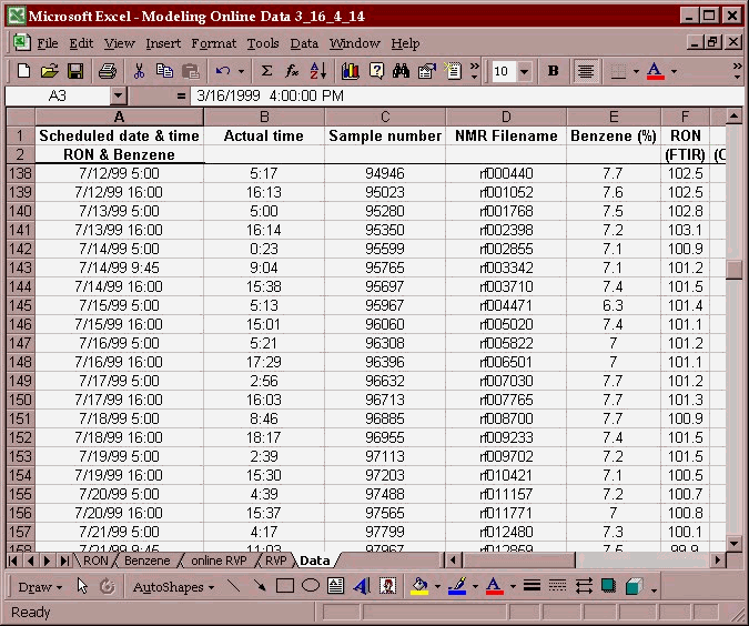
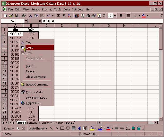
The data is placed in individual columns matching a parameter with the associated spectral file. The two columns are then copied to the clipboard:
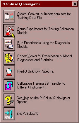
The data is then transferred into the PLS/IQ software and a calibration development file (*.tdf) is created.
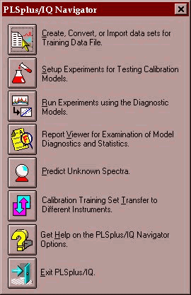
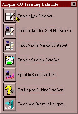
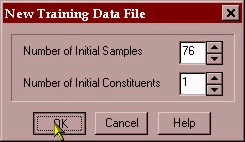
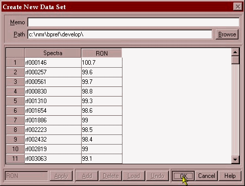
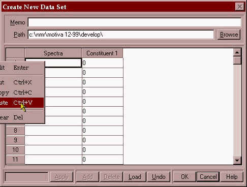
We will save this file as ron-demo.tdf. We then open this development file and begin the PLS modeling.
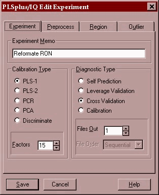
The PLS-1 algorithm will be used and a 15 factor model will be created using a leave-1-out cross validation. This means that the model is built 76 times with 75 of the samples leaving a different sample out every time. The sample left out is then predicted by the model and an error value is obtained for the model containing 1 factor, 2 factors – up to 15 factors. This residual error is then used to decide the optimum number of factors to use in the model.
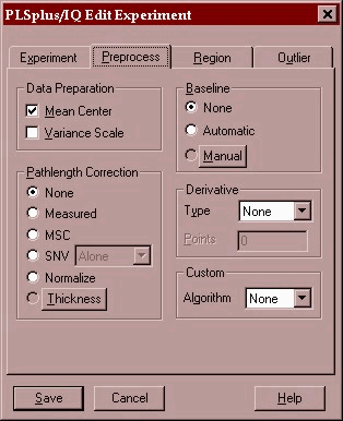
The only preprocessing performed is a mean centering of the data. This is when the average spectrum of all 76 samples is subtracted from each of the spectra. This allows the PLS algorithm to operate on the true spectral variance in the data set.
The model algorithm is now run:
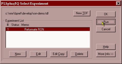
After the program has run we enter the report reader component of the PLS/IQ software.
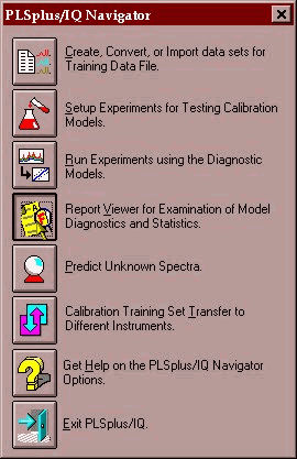
The appropriate *.tdf file is chosen and the model is picked from the list of possibilities.
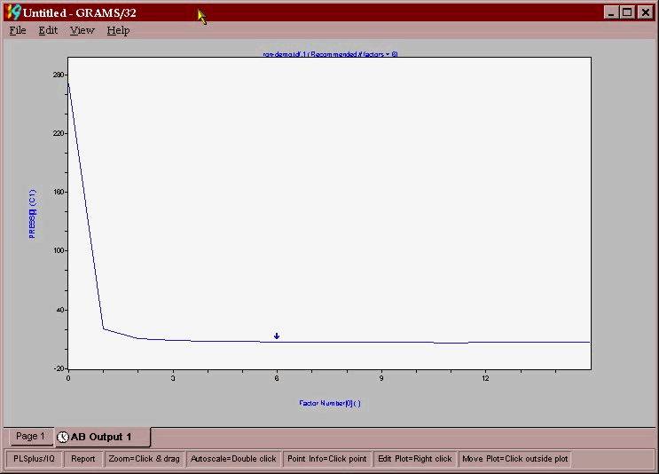
The first screen that is shown is the PRESS versus factor number plot. PRESS is the Prediction Residual Error Sum of Squares, and represents the error between the lab value and the NMR prediction for a model containing a given number of factors. Where this error reaches a minimum in the PRESS versus “number of factors” plot is a strong indicator of the optimum number of factors that one should use in the calibration. The figure below shows the PRESS/Factor plot for reformate RON model. The Grams software performs a number of statistical significance tests and indicates that 6 factors is the optimum number of significant factors.
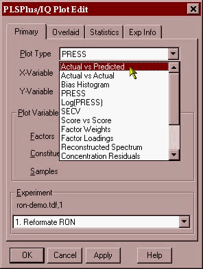
The task is now to ascertain if any outliers are present in the data set. The plot below shows the actual lab value plotted against the NMR predicted value using a 6-factor calibration. The various plots that one uses for reports or outlier detection diagnostics are obtained by left clicking on the plot and picking the plot you want from the drop down menu that appears (shown here).
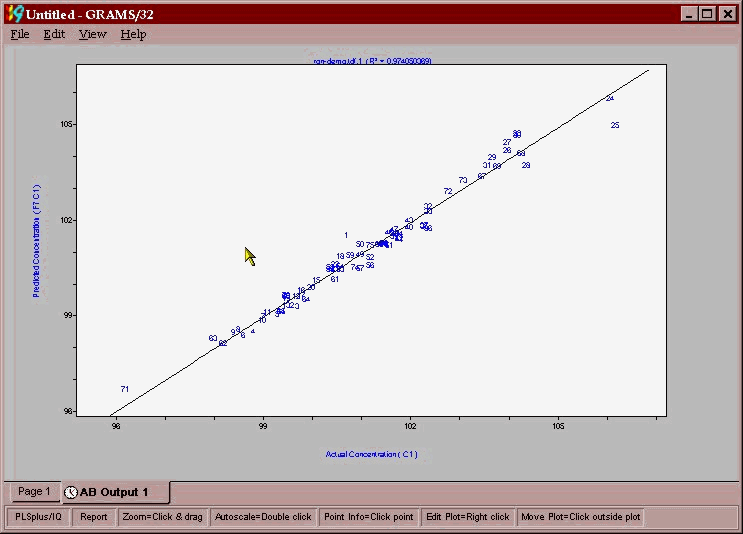
From this plot it appears that 25 is a possible outlier while 24 and 71 would have a large leverage on the model (some samples can have an overly large impact on the model) and may need to be excluded because of this. A good indicator of outliers is the leverage versus studentized residual plot.(shown below) samples with high leverage or studentized residuals > 2.5 should be removed as outliers.
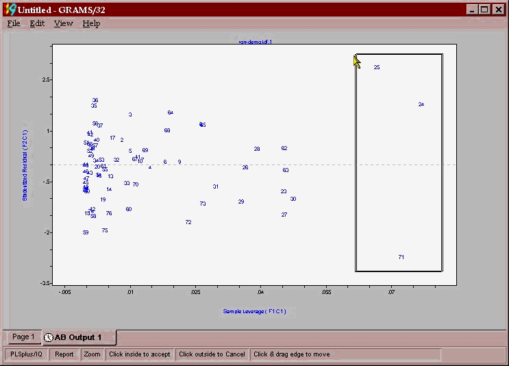
These samples are then excluded and the whole modeling process performed again to yield the model depicted below in a combined PRESS/factor and actual/predicted plot.
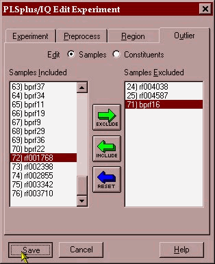
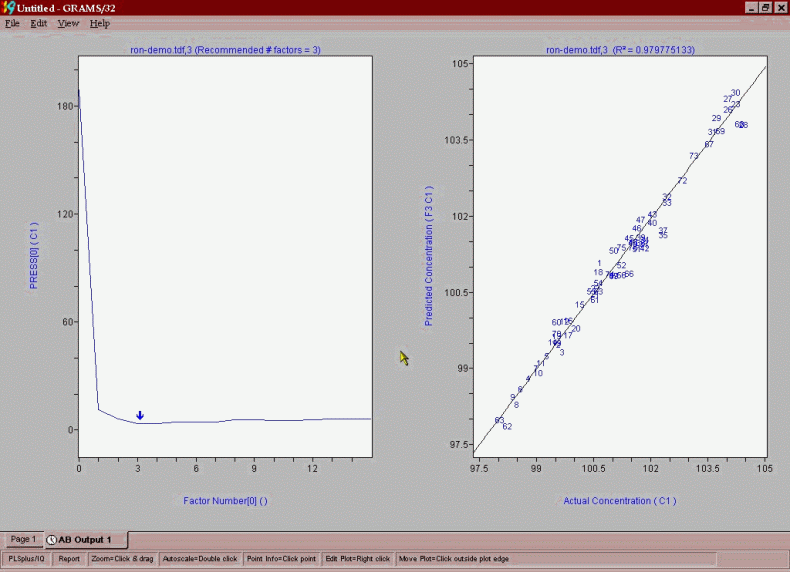
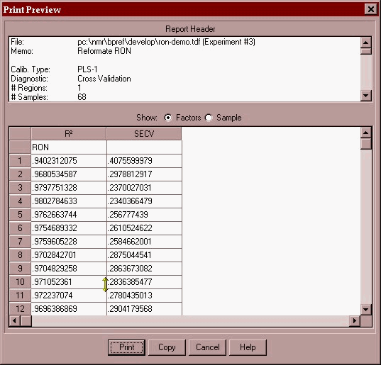
Now that we are happy there are no more outliers and the error between lab and NMR is within tolerance (0.23 octane numbers) we can print a report and save the PLS model as a calibration file (*.cal).
This calibration file can then be transferred to the Foxboro NMR spectrometer and be used to predict the RON on-line.
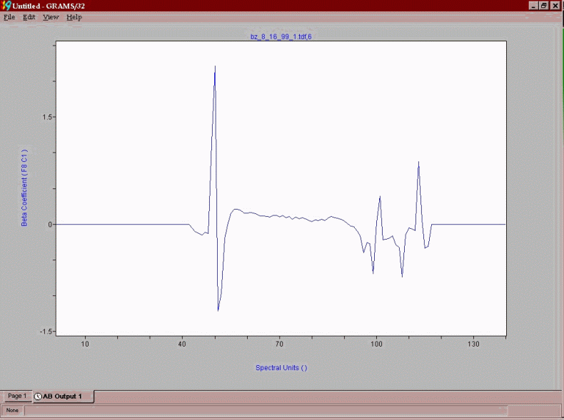
The final product of the chemometric modeling effort is a predictive vector that is a series of coefficients that each point in the spectrum is multiplied by to yield a process control number, such as RON, MON, Benzene. A predictive vector for RON in reformate is shown below. The positive points in the vector correlate to chemistry that positively impacts RON and negative regions are relatable to negative impacting chemistry.
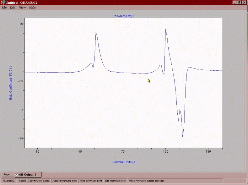
As can be seen, aromatics are a large positive contributor, while paraffinic components are generally negatively impacting on RON. The vector for benzene content in Vol% is shown below:
